Apps
The Apps button in the top bar opens a panel with tools that work on the current view and its tracks. Click an entry to open it; the arrow at the top left of the panel goes back to the list of apps, and Esc or the red X closes the panel.
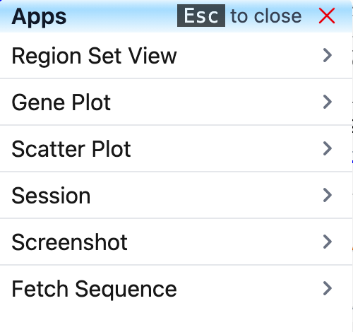
The panel lists:
- Region Set View: view a list of genes or regions side by side.
- Gene Plot: summarize a numerical track over a gene or region set.
- Scatter Plot: compare two numerical tracks over a gene or region set.
- Session: save, share and load sessions.
- Screenshot: export the current view as an SVG or PDF image.
- Fetch Sequence: get the genomic sequence of the view or of a list of regions.
The previous version of the Browser also had a Go Live app, which mirrored your view on the screens of others in real time. This version does not have it.
Region Set View
A region set is a list of genes and/or genomic regions. The Browser can show all the regions of a set next to each other in one view, so you can compare the same tracks across many loci at once. Region sets are also the input of Gene Plot and Scatter Plot. They are kept in the current session.
Create a set
-
Click Apps, then Region Set View, then Add New Set.
-
In the Create New Set box, enter gene names or coordinates, one per line. Gene names and coordinates can be mixed. Coordinates must be in the form
chr1:345-678.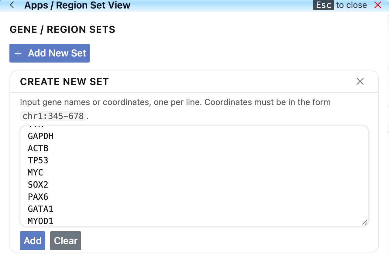
-
Click Add. The Browser looks up each gene in the current genome and shows the set editor. Clear empties the text box.
If any line cannot be found in the genome (a misspelled gene name, for example), the set is not created and the editor does not appear; no message says which line failed. Check the names and click Add again.
Edit the set
The editor has three parts:
- Set name: type a name for the set. The name is how you choose the set later in Gene Plot and Scatter Plot.
- Add or remove regions: add one more region by giving a Name and a Locus and clicking Add, or click Add Multiple to paste another list of genes or coordinates. Each row of the table has a Delete link. Click a column header to sort the table.
- Set flanking region: choose which part of each feature to view, and how much sequence to add around it. Surrounding can be Whole region, Region start or Region end; Upstream bases and Downstream bases set how many bases to add on each side. Start, end, upstream and downstream follow the strand of each feature. The Coordinates to view column shows the result.
By default, features on the minus strand are flipped so that every region reads from 5' to 3'. Check No flip for regions on - strand to keep them in genome orientation.
In this example, 12 genes are viewed as their promoters: 2,000 bases upstream and downstream of the gene start (Region start).
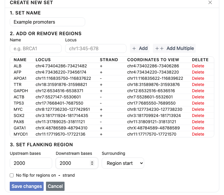
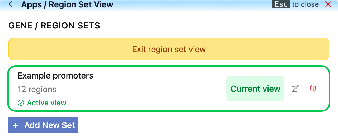
Click Save changes to add the set, or Cancel to discard it. The set then appears in the list:
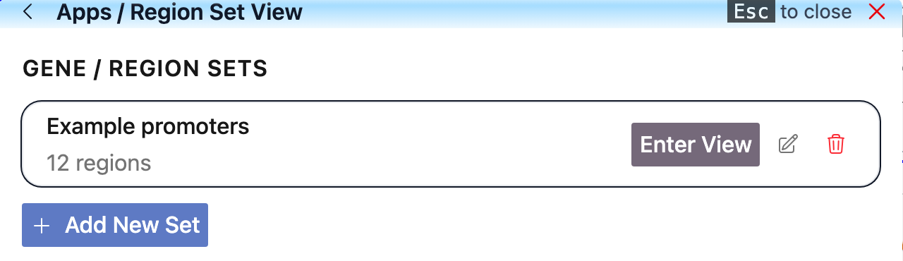
To change a set later, click its pencil icon (Edit set); to remove it, click the trash icon (Delete set).
Enter and exit the region set view
Click Enter View next to a set. The set is marked Current view and Active view, and an Exit region set view button appears at the top of the panel.
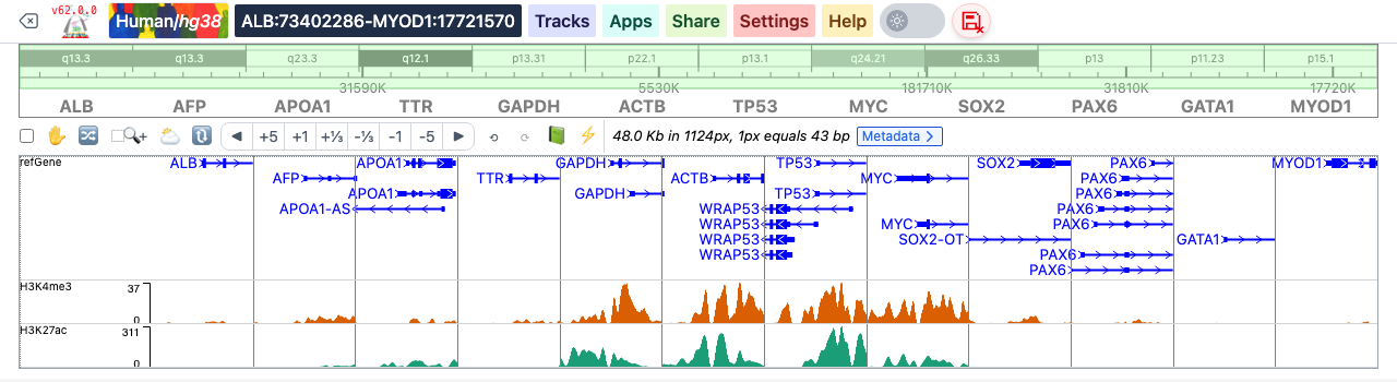
Close the panel to see the result: the regions are shown next to each other, in the order of the set, with their names above the tracks. The box in the top bar shows the span from the first to the last region.
To go back to the normal genome view, open Apps > Region Set View and click Exit region set view.
Gene Plot
Gene Plot shows the overall signal of a numerical track over a gene or region set. Each region (after flanking, see Edit the set) is split into the same number of bins, read 5' to 3' relative to its strand, and the track's average value in each bin is computed. Only tracks of type bigwig and bedgraph that are in the current view can be chosen.
- Click Apps, then Gene Plot. If the session has no region set yet, the panel says so and shows the region set tools, so you can create one first.
- 1. Region Set: choose the set.
- 2. Numerical Track: choose the track.
- 3. Plot Options: choose the Plot type (box, line or heatmap) and the number of Data points (bins per region, 50 to 100).
- Click Plot. "Loading..." shows while the data are fetched; the plot appears below.
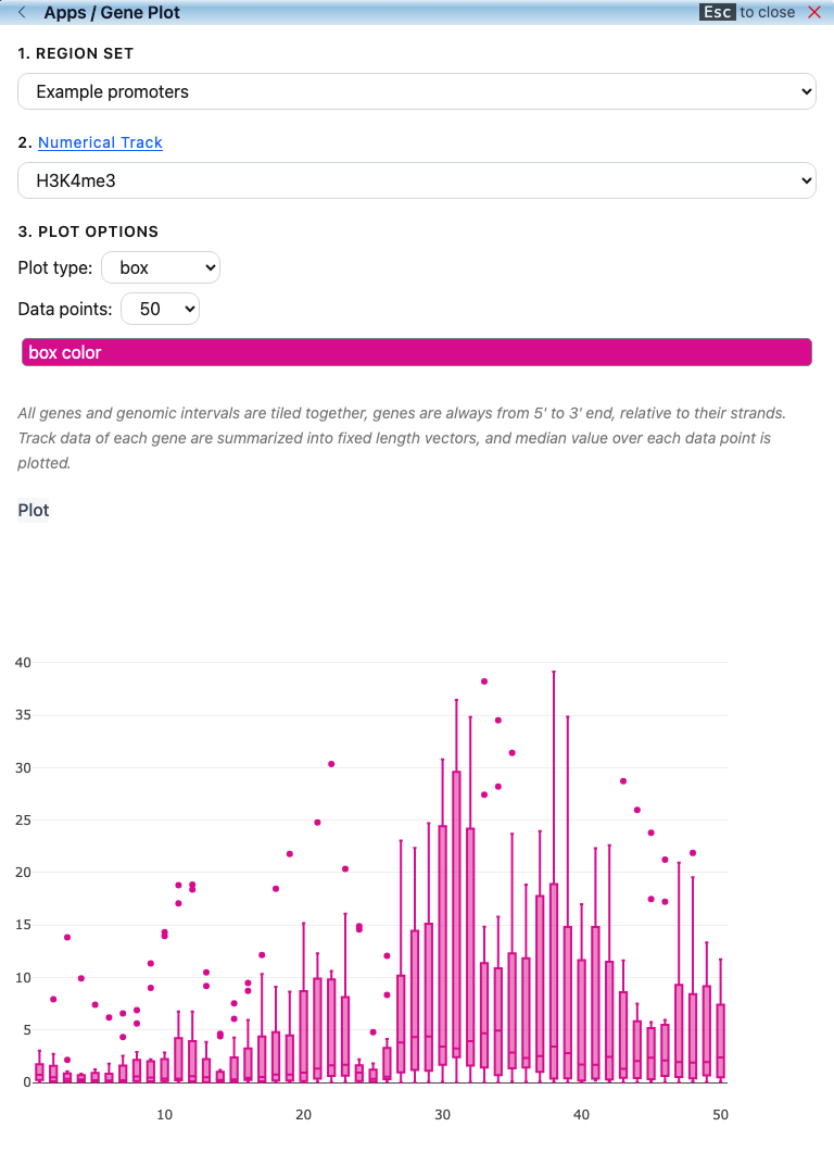
The box plot has one box per bin, summarizing the values of all regions in that bin. Once a box plot is drawn, a box color button lets you change the color of the boxes. Below, the H3K4me3 signal over the 12 promoters of the example set peaks around the gene starts (the middle of the 4 kb windows):
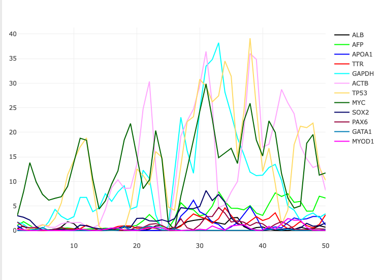
The line plot draws one line per region, with a legend of the region names:
The heatmap draws one row per region:
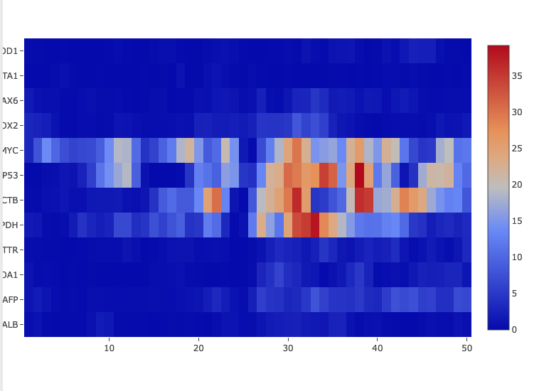
Changing the plot type redraws the same data; click Plot again after changing the set, the track or the number of data points. A short description of each plot type is shown above the Plot button.
When you move the mouse over the plot, a tool bar appears at its top right. The camera icon (Download plot) saves the plot as an SVG file; the other icons zoom, pan and reset the axes.

The plot area is wider than the panel and its left edge is cut off, so the region names of the heatmap are only partly visible. Downloading the plot gives the full image.
Scatter Plot
Scatter Plot compares two numerical tracks over a gene or region set: each region of the set is one point, placed at the mean of each track's values in that region (X track on the horizontal axis, Y track on the vertical axis). The Pearson correlation of the two tracks over the set is shown above the plot as R.
- Click Apps, then Scatter Plot. As with Gene Plot, you need a region set first.
- 1. Region Set: choose the set.
- 2. Numerical Track (X-axis) and 3. Numerical Track (Y-axis): choose the two tracks (
bigwigorbedgraphtracks in the view). - 4. Plot Configuration: set the Marker color and Marker size.
- Click Plot.
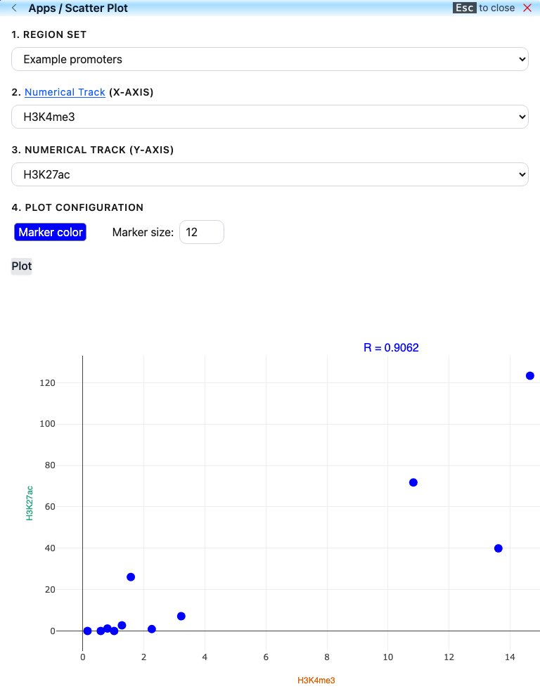
Hovering over a point shows its two values and the region name. The plot's tool bar (camera icon) downloads the plot as an image.
Session
Apps > Session offers the same tools as the Save/Load Session tab of the session panel: retrieve a saved session bundle by its ID, upload a session file, save the current view remotely to get a bundle ID you can share, and download the current session or its tracks as a JSON file.
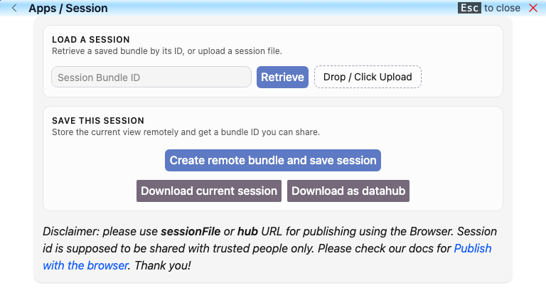
All of this is described in Manage sessions.
Screenshot
The Screenshot app re-draws the tracks of the current view as a vector image, for figures in papers and presentations.
- Navigate to the region you want and set up the tracks.
- Click Apps, then Screenshot. The panel shows the re-drawn view, with the track names on the left.
- Click Download SVG or Download PDF. The file is named with the date and time, for example
2026-11-21T02:25:58.876Z_eg.svg.
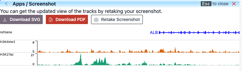
The image is taken when the app opens. If you change the view while the panel is open, click Retake Screenshot to update it. If there are no tracks in the view, the panel shows "No tracks in view".
Fetch Sequence
Fetch Sequence gets the genomic DNA sequence, in FASTA format, of the current view or of a list of regions. It works for genomes that have a sequence file; otherwise it says "Genomic sequence is not added to this genome yet."
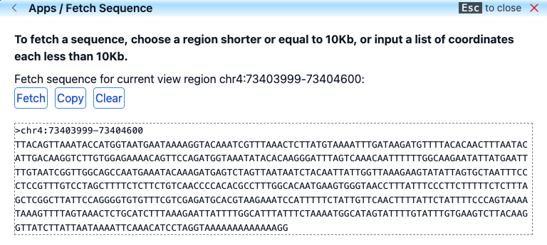
Sequence of the current view
- Navigate to the region you want. Keep it at 10 kb or less.
- Click Apps, then Fetch Sequence. The panel names the current region.
- Click Fetch. The sequence appears below; Copy copies it to the clipboard and Clear removes it.
Sequences of a list of regions
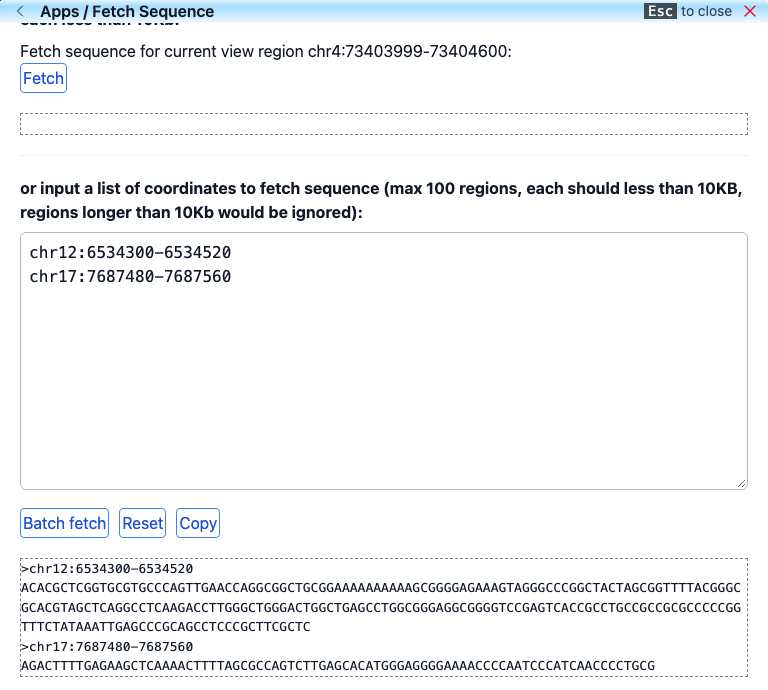
- In the box below, enter up to 100 coordinates, one per line, for example
chr12:6534300-6534520. Regions longer than 10 kb are skipped (they come back with an empty sequence). - Click Batch fetch. Each region is returned as a FASTA record. Copy copies them all, and Reset empties the box.
The 10 kb limit is only enforced for the list. Fetch for the current view also returns longer regions, but a long sequence makes the panel slow to use.